Python【探空订正】效果

付亚男 · 发表于 2023-6-16 00:48:30

登录后查看更多精彩内容~

您需要登录才可以下载或查看，没有帐号？立即注册

x

本帖最后由付亚男于 2026-9-9 10:12 编辑

   MICAPS的交互探空有一个很实用的效果——修正抬升点。对于早晨08时的探空，可以通过将地面温度和露点加以订正，考察午后的对流潜势。另外在近地面是稳定层结时，通过将抬升点提高到稳定层结以上，可以考察高架对流发生的可能性。
   MetPy提供了一个功能丰富的绘制探空图的函数：Advanced Sounding — MetPy 1.5 (unidata.github.io)。其本质就是在图上绘制各种线条（温度廓线、露点廓线、状态曲线等），各种点（LCL、LFC、EL）以及填色区（CAPE和CIN）。那么实现MICAPS的交互探空功能，其实就是在原图上取一个新的抬升点、计算一条新的状态曲线以及LCL和LFC，填上新的CAPE和CIN颜色。
   了解了原理，就很容易实现了。

Figure 2023-06-16 003750.png

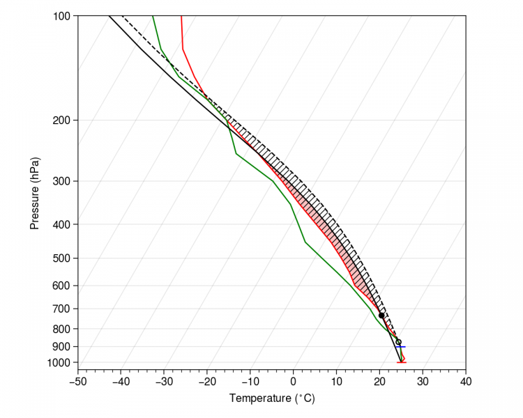
   上面这张图就是绘制的效果，红线和绿线分别是温度廓线和露点廓线。
   黑色实线是基于1000 hPa抬升的状态曲线，对应的LFC高度以黑色实心点标注，CAPE以半透明红色进行填色。
   黑色虚线是基于900 hPa抬升的状态曲线，对应的LFC高度以黑色空心点标注，CAPE为斜线填充区域。
   为了方便考察LFC距离抬升点的位置，把抬升点以短横线标注出来，红色基于1000 hPa，蓝色基于900 hPa。

   这张探空取自一个比较典型的高架对流的探空：最不稳定层在900-875 hPa，这一层次CAPE大约是1200 J/kg，地面约为500 J/kg；CIN在这一层次为0；从这一层次抬升，只需要抬升很短的距离，就可以到达LFC，从而出现自由对流，而从地面抬升，需要抬升约3000 m才能出现自由对流；当然之所以判断对流是高架的，还有一点在这里没有展示，就是地面图中这个位置附近没有明显的辐合特征。

   代码不复杂，按照上面的思路，很容易实现。设置回复可见以便更多人可以看到。测试数据是自己写的npy，一并给出。

# -*- coding: utf-8 -*-
'''
Author : fuyanan
Created on : Thu Jun 15 11:32:54 2023
Description :
two parcel profiles from different levels in one T-lnP
'''
# %%
import numpy as np
from metpy import calc
from metpy.units import units
from metpy.plots import SkewT
import matplotlib.pyplot as plt
import proplot as pplt
# %%
npyf = np.load(r'E:/python/testdata/ForTlnP.npy')
pressure = npyf[0]*units('hPa')
temperature = npyf[1]*units('K')
relative_humidity = npyf[2]*units('%')
dewpoint = calc.dewpoint_from_relative_humidity(temperature, relative_humidity)
# %%
def PlotProfile(skew, pressure, temperature, dewpoint, order):
# plot parcel profile
parcel_prof = calc.parcel_profile(
pressure, temperature[0], dewpoint[0],
).to('degC')
skew.plot(
pressure,
parcel_prof,
linewidth = 1,
linestyle = '-'if order==0 else '--',
color='k',
)
# plot LFC
lfc_pressure, lfc_temperature = calc.lfc(
pressure, temperature, dewpoint, parcel_prof, dewpoint[0],
)
skew.plot(
lfc_pressure,
lfc_temperature,
'ko',
markerfacecolor = 'k' if order==0 else 'none',
markeredgecolor = 'k',
markersize = 4,
)
# shade cape
skew.shade_cape(
pressure,
temperature,
parcel_prof,
facecolor = 'red' if order==0 else 'w',
hatch = None if order==0 else '/////',
)
# plot root
skew.plot(
pressure[0],
temperature[0].to('degC'),
marker = '_',
markersize = 8,
markeredgecolor = 'r' if order==0 else 'b',
)
return None
def TlnP_DoubleParcel(pressure, temperature, dewpoint, second_level):
fig = plt.figure(figsize=(6, 4.8),facecolor='w')
skew = SkewT(fig, rotation=30)
skew.plot(pressure, temperature, 'r', lw=1)
skew.plot(pressure, dewpoint, 'g', lw=1)
skew.ax.set_ylim(1050, 100)
skew.ax.set_xlim(-50, 40)
PlotProfile(
skew,
pressure,
temperature,
dewpoint,
order=0,
)
PlotProfile(
skew,
pressure[pressure<=second_level],
temperature[pressure<=second_level],
dewpoint[pressure<=second_level],
order=1,
)
skew.ax.set_xlabel(r'Temperature ($^\circ$C)')
skew.ax.set_ylabel(r'Pressure (hPa)')
plt.tight_layout()
return None
# %%
TlnP_DoubleParcel(pressure, temperature, dewpoint, second_level=900*units('hPa'))

复制代码

ForTlnP.npy (1016 Bytes, 下载次数: 91)

勿忘草 · 发表于 2023-6-16 08:39:54

好东西，学习了

道狼52203 · 发表于 2023-6-16 09:51:34

{:eb511:}

流浪的心 · 发表于 2023-6-16 10:11:28

感谢分享！

随缘 · 发表于 2023-6-16 11:05:22

设置回复可见以便更多人可以看到

Zhu-xrui-1 · 发表于 2023-6-16 11:23:59

谢谢，学习了

跺碎那片云 · 发表于 2023-6-16 13:22:50

{:eb348:}

水木缘 · 发表于 2023-6-16 15:48:44

{:5_213:}

tulalang · 发表于 2023-6-16 21:09:54

胖爷威武~

东水兽 · 发表于 2023-6-17 09:23:45

考察午后的对流潜势？有相关的文章么

		自动登录	找回密码
密码			立即注册

[经验总结] Python【探空订正】效果

登录后查看更多精彩内容~